Overview
This post will go over many of the ways in which to set plot colors while using Matplotlib. We'll also walk through using the built-in Matplotlib colormaps.
A Basic Plot
We'll first go over setting colors in a manual and straightforward way.
By default, each time you plot a new layer or axis in Matplotlib, it will use a new color.
from matplotlib import pyplot as plt
import numpy as np

x = np.arange(0, 10, 0.2)

# Every time plot is called, the color cycler iterates.
plt.plot(x, x)
plt.plot(x, x**1.5)
plt.plot(x, x**2)
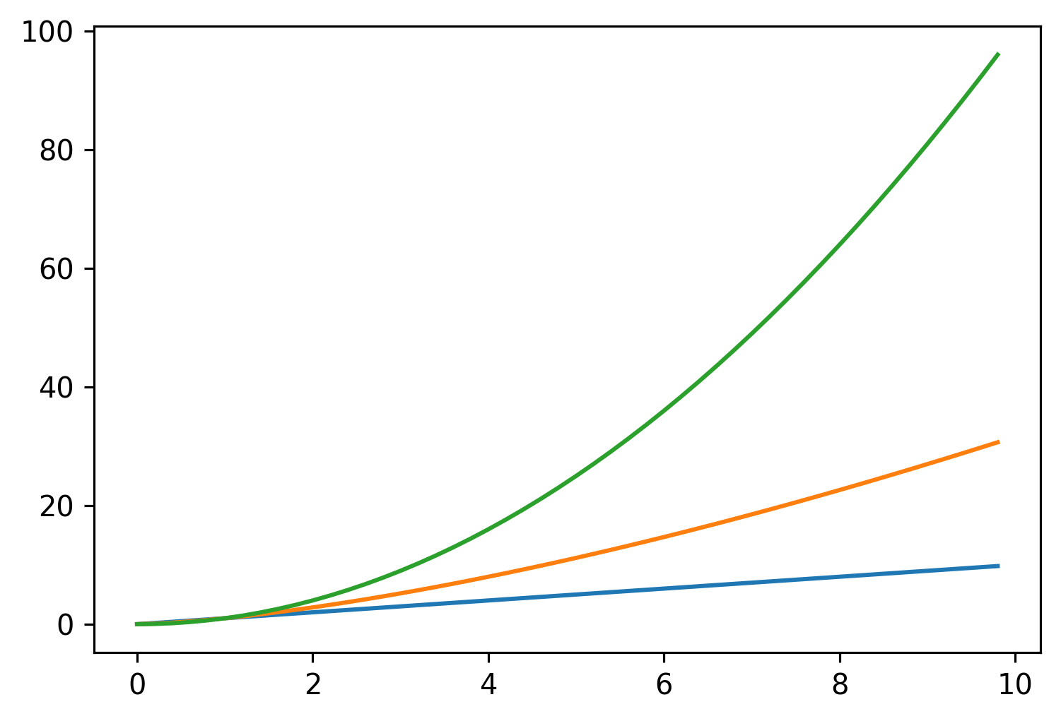
These colors come from the default color cycler, which we can see in the plot config:
print(plt.rcParams['axes.prop_cycle'])
# Output:
# cycler('color', ['#1f77b4', '#ff7f0e', '#2ca02c', '#d62728', '#9467bd', '#8c564b', '#e377c2', '#7f7f7f', '#bcbd22', '#17becf'])
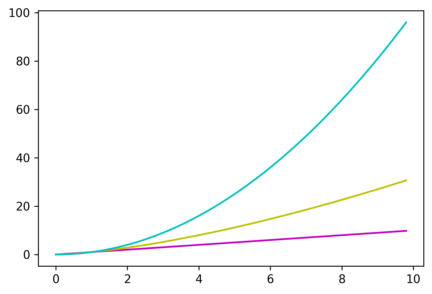
You can also explicitly set colors, via the fmt positional argument or the color keyword argument.
plt.plot(x, x, 'm')  # shorthand for magenta
plt.plot(x, x**1.5, 'y')  # shorthand for yellow
plt.plot(x, x**2, 'c')  # shorthand for cyan
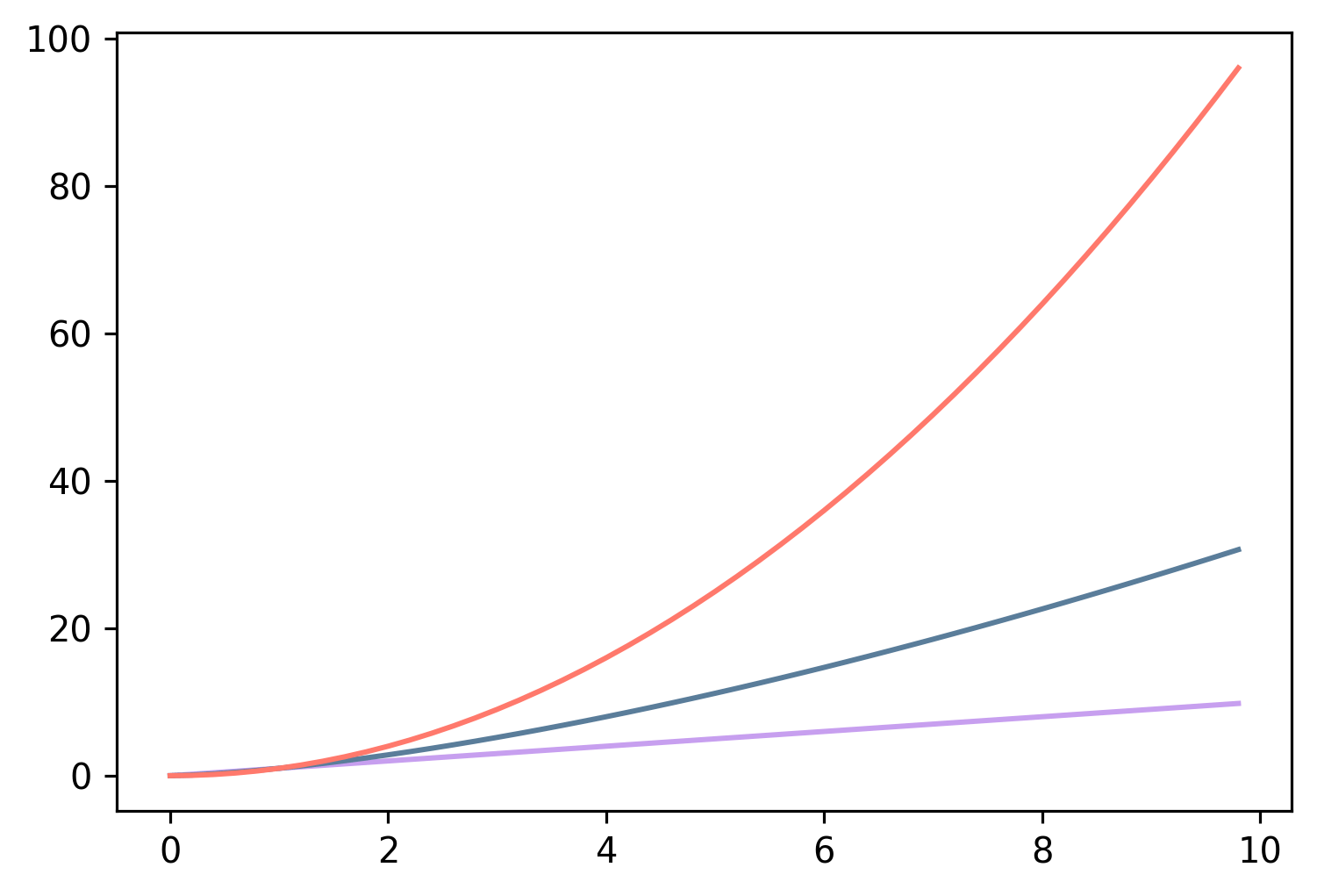
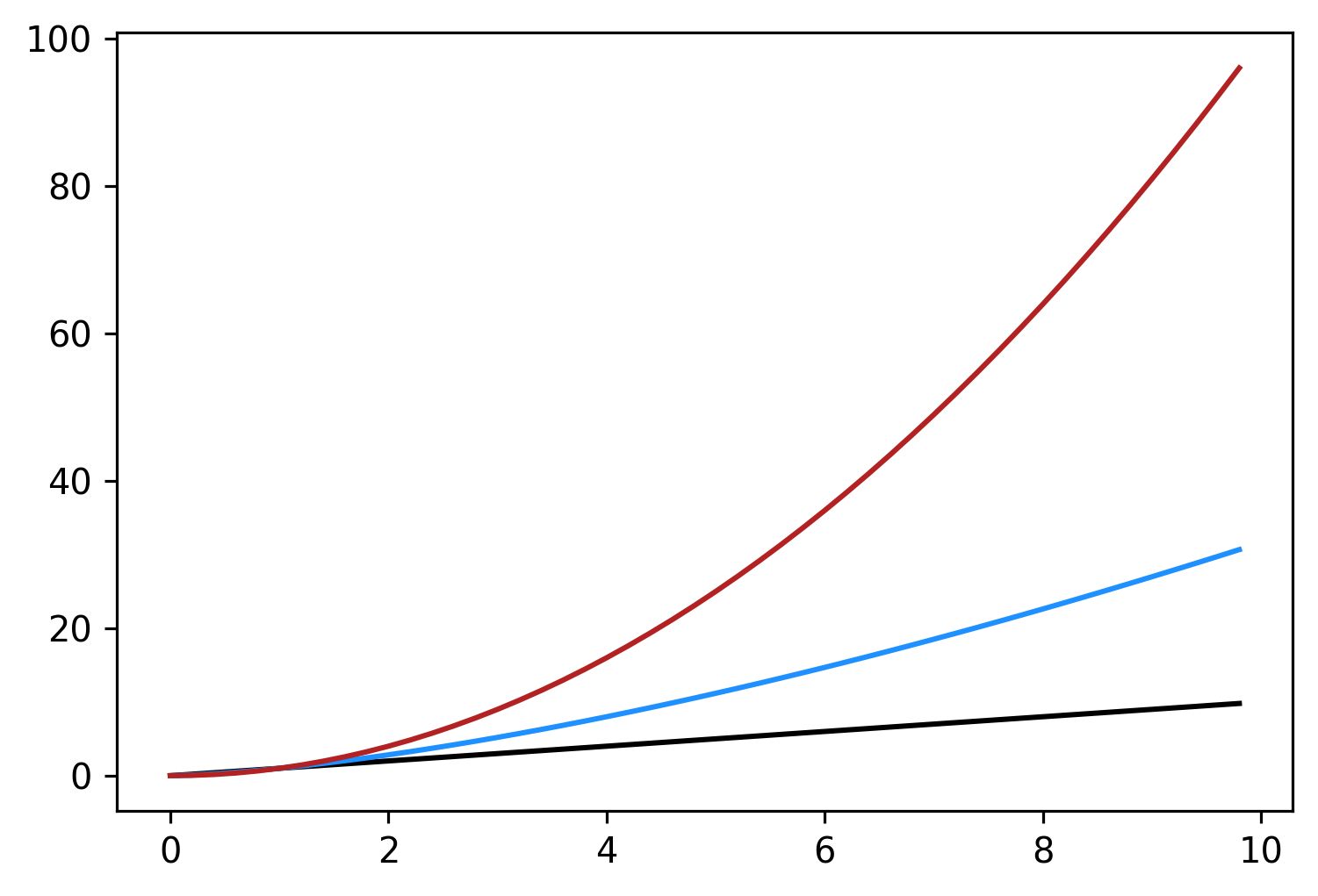
Alternatively, you can use the color argument:
plt.plot(x, x, color='#c79fef')
plt.plot(x, x**1.5, color='#5a7d9a')
plt.plot(x, x**2, color='#ff796c')
Everything above is available via ax.plot as well if using the object-oriented approach via plt.subplots().
Color Cyclers
Instead of manually specifying the color for every line, we can set a color cycler before we plot anything, and each
axis will sequentially be given the next color.
plt.rcParams['axes.prop_cycle'] = plt.cycler(
    color=['black', 'dodgerblue', 'firebrick'])

plt.plot(x, x)  # Will be black
plt.plot(x, x**1.5)  # dodgerblue
plt.plot(x, x**2)  # firebrick
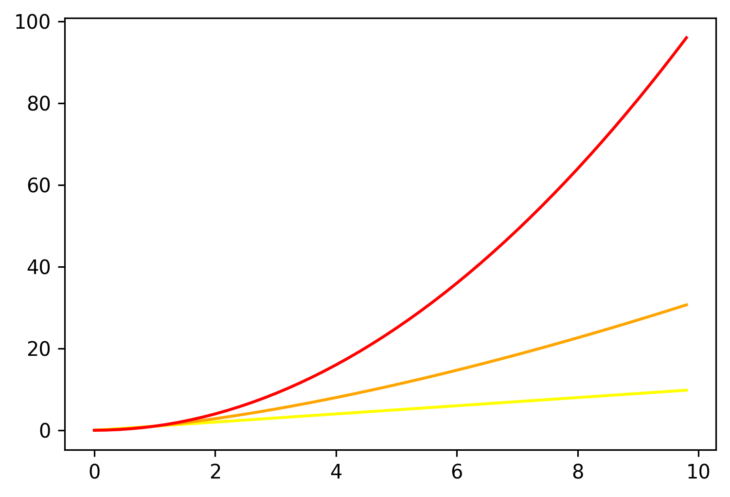
For a more object-oriented approach, it's better to set the prop_cycle via the Axes object, as below. That way you
don't have to mess with the global config settings.
fig, ax = plt.subplots()
ax.set_prop_cycle(color=['yellow', 'orange', 'red'])
ax.plot(x, x)
ax.plot(x, x**1.5)
ax.plot(x, x**2)
Colormaps
Lastly, we'll explore built-in colormaps in Matplotlib. The library has some great documention on this which you should check out as well:
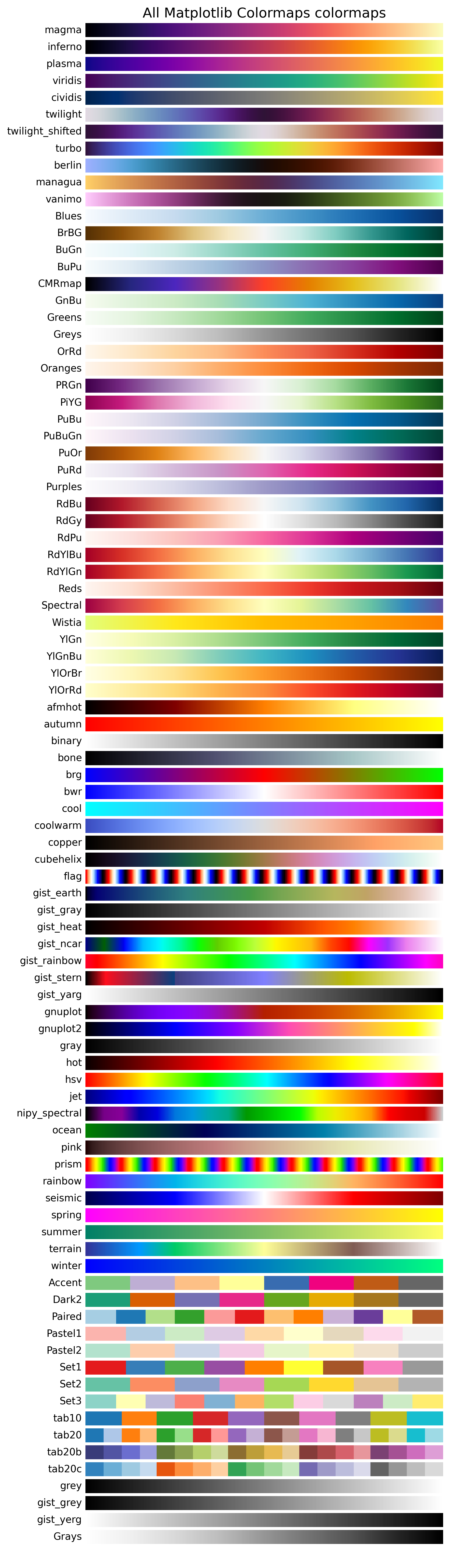
Colormaps are preset lists/sequences/maps of colors that Matplotlib already has packaged up for us, ready to use. To see all available color maps, you can use the command below (or look at the second link above):
from matplotlib import colormaps
list(colormaps)
# Output: a long list of colormaps!
You can also plot each of them out if you'd like, using a helper function like the below:
import matplotlib as mpl
from matplotlib import pyplot as plt
import numpy as np

cmaps = {}

gradient = np.linspace(0, 1, 256)
gradient = np.vstack((gradient, gradient))


def plot_color_gradients(category, cmap_list):
    # Create figure and adjust figure height to number of colormaps
    nrows = len(cmap_list)
    figh = 0.35 + 0.15 + (nrows + (nrows - 1) * 0.1) * 0.22
    fig, axs = plt.subplots(nrows=nrows + 1, figsize=(6.4, figh))
    fig.subplots_adjust(top=1 - 0.35 / figh, bottom=0.15 / figh,
                        left=0.2, right=0.99)
    axs[0].set_title(f'{category} colormaps', fontsize=14)

    for ax, name in zip(axs, cmap_list):
        ax.imshow(gradient, aspect='auto', cmap=mpl.colormaps[name])
        ax.text(-0.01, 0.5, name, va='center', ha='right', fontsize=10,
                transform=ax.transAxes)

    # Turn off *all* ticks & spines, not just the ones with colormaps.
    for ax in axs:
        ax.set_axis_off()

    # Save colormap list for later.
    cmaps[category] = cmap_list

# Get all colormaps except the reversed ones, which are suffixed with "_r".
non_reversed_colormaps = [colormap for colormap in list(colormaps)
    if not colormap.endswith('_r')]
plot_color_gradients('All Matplotlib Colormaps', non_reversed_colormaps)
Using a Colormap
Now that we know and can see all the colormaps available to us, how do we use them? Colormaps are accessible in many ways in Matplotlib, here are a few:
# Using previous imports...

# Via the most recent documentation, this first option seems to be recommended.
viridis = mpl.colormaps['viridis']
viridis = plt.get_cmap('viridis')
viridis = plt.cm.viridis
There are a few ways you can then use that viridis object. The first is just to call it as a function, with a list as
an argument, and values between 0 and 1 within that list. Each list value will return a color from the colormap; the
closer the value is to zero, the closer to the "left" the color returned will be, and a value of 1 will give the last
color on the far "right". The colors are returned in RGBA format - Red, Green, Blue, Alpha (transparency), and these
can be directly used in the ways already discussed in this post.
viridis = mpl.colormaps['viridis']
# This will give us 5 colors, evenly dispersed
viridis([0, 0.25, 0.5, 0.75, 1])

# Outputs an array of colors in RGBA format:
# array([[0.267004, 0.004874, 0.329415, 1.      ],
#        [0.229739, 0.322361, 0.545706, 1.      ],
#        [0.127568, 0.566949, 0.550556, 1.      ],
#        [0.369214, 0.788888, 0.382914, 1.      ],
#        [0.993248, 0.906157, 0.143936, 1.      ]])
It's worth noting, there are two types of colormaps, with slightly different functionality: ListedColormaps and
LinearSegmentedColormaps.
Directly from the documentation:
ListedColormaps store their color values in a .colors attribute. The list of colors that comprise the colormap can be directly accessed using thecolorsproperty, or it can be accessed indirectly by callingviridiswith an array of values matching the length of the colormap. Note that the returned list is in the form of an RGBA (N, 4) array, where N is the length of the colormap.
LinearSegmentedColormaps do not have a .colors attribute. However, one may still call the colormap with an integer array, or with a float array between 0 and 1.
So, to fetch colors from a ListedColormap, you can do:
# Get all colors.
viridis.colors
# Get the first 8 colors.
viridis(range(8))
# Get 8 colors, evenly distributed.
viridis(np.linspace(0, 1, 8))
# Get 8 colors, evenly distributed.
viridis.resampled(8).colors
Note the usage of resampled in the last example above. That function is available on both colormap types, and
basically returns a colormap with N underlying colors, evenly distributed within the colormap. For ListedColormaps,
it's a slightly nicer way to get evenly distributed colors vs using the np.linspace() method.
For a LinearSegmentedColormap, you'd access in similar ways, but the colors attribute is not available, so really
the two options are:
copper = mpl.colormaps['copper']
print(type(copper))
# First 8 colors.
print(copper(range(8)))
# 8 colors, evenly distributed.
print(copper(np.linspace(0, 1, 8)))
# 8 colors, evenly distributed.
print(copper.resampled(8)(range(8)))

# Output:
# <class 'matplotlib.colors.LinearSegmentedColormap'>
# [[0.         0.         0.         1.        ]
# [0.00484429 0.00306353 0.00195098 1.        ]
# [0.00968858 0.00612706 0.00390196 1.        ]
# [0.01453287 0.00919059 0.00585294 1.        ]
# [0.01937716 0.01225412 0.00780392 1.        ]
# [0.02422145 0.01531765 0.0097549  1.        ]
# [0.02906574 0.01838118 0.01170588 1.        ]
# [0.03391003 0.02144471 0.01365686 1.        ]]
# [[0.         0.         0.         1.        ]
# [0.17439442 0.11028706 0.07023529 1.        ]
# [0.35363313 0.22363765 0.14242157 1.        ]
# [0.52802756 0.33392471 0.21265686 1.        ]
# [0.70726627 0.44727529 0.28484314 1.        ]
# [0.88166069 0.55756235 0.35507843 1.        ]
# [1.         0.67091294 0.42726471 1.        ]
# [1.         0.7812     0.4975     1.        ]]
# [[0.         0.         0.         1.        ]
# [0.17647055 0.1116     0.07107143 1.        ]
# [0.35294109 0.2232     0.14214286 1.        ]
# [0.52941164 0.3348     0.21321429 1.        ]
# [0.70588219 0.4464     0.28428571 1.        ]
# [0.88235273 0.558      0.35535714 1.        ]
# [1.         0.6696     0.42642857 1.        ]
# [1.         0.7812     0.4975     1.        ]]
So, very similar, but without the convenice colors attribute.
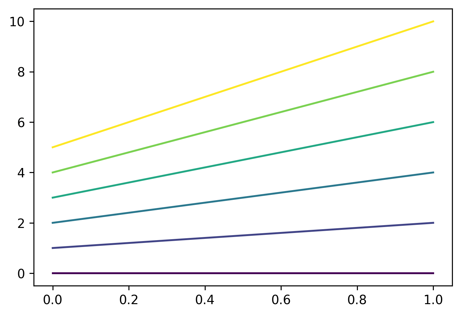
Let's now put this all into action.
N = 6
fig, ax = plt.subplots()
ax.set_prop_cycle(color=viridis(np.linspace(0, 1, N)))
for i in range(N):
    ax.plot([0, 1], [i, 2 * i])
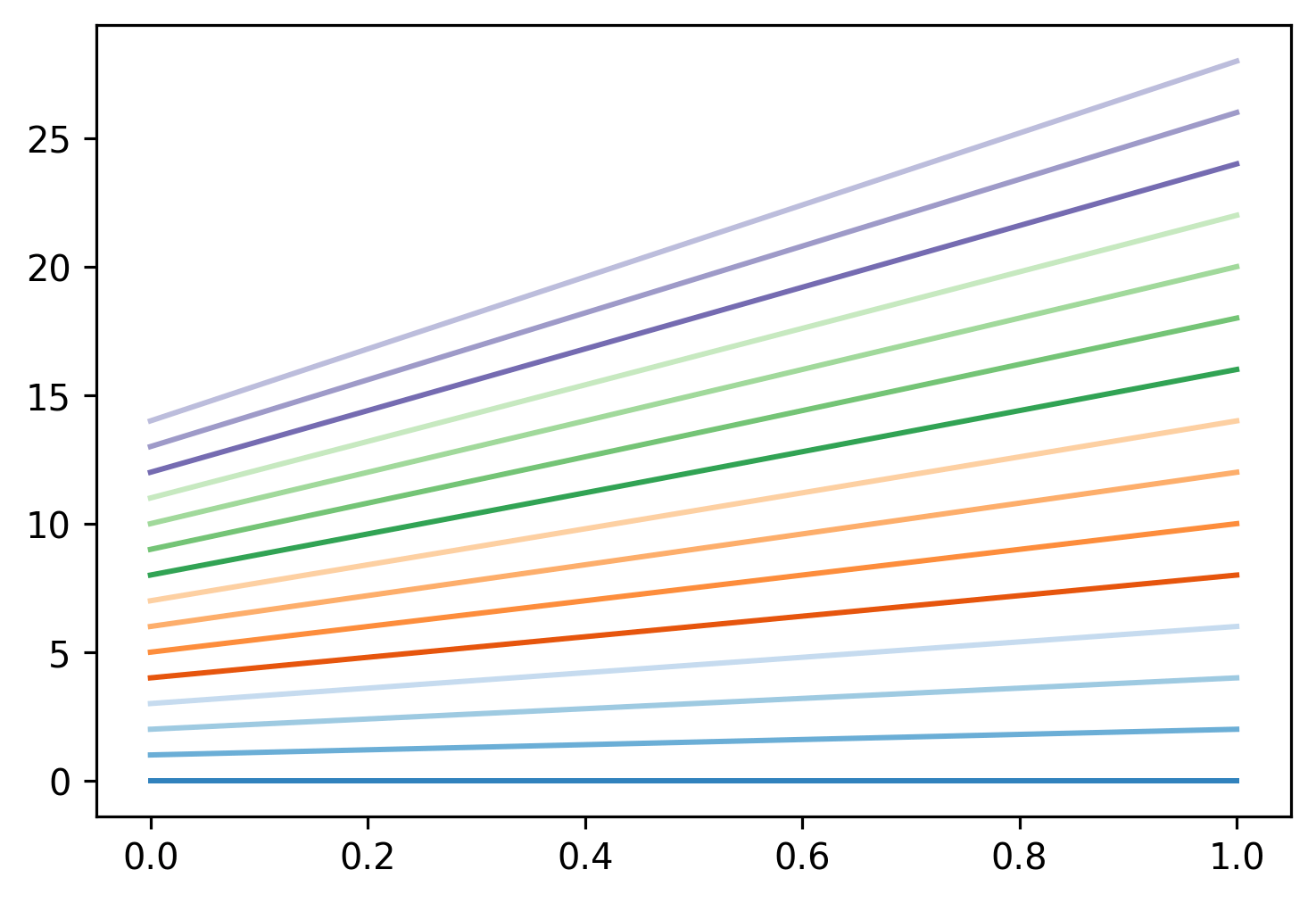
Now an example using a qualitative colormap, cycling through each color in order:
N = 15
fig, ax = plt.subplots()
ax.set_prop_cycle(color=mpl.colormaps['tab20c'](range(N)))
for i in range(N):
    ax.plot([0,1], [i, 2*i])
plt.show()
We can get the same thing using .colors:
N = 15
fig, ax = plt.subplots()
ax.set_prop_cycle(color=mpl.colormaps['tab20c'].colors[:N])
for i in range(N):
    ax.plot([0,1], [i, 2*i])
plt.show()

We can define a helper function if we'd like, although maybe not necessary given how short/easy this is..
def set_sequential_palette(ax, name='Blues', start=0, stop=1, n=8):
"""Set seqential colors for a Matplotlib plot"""
ax.set_prop_cycle(color=mpl.colormaps[name](np.linspace(start, stop, n)))
return ax
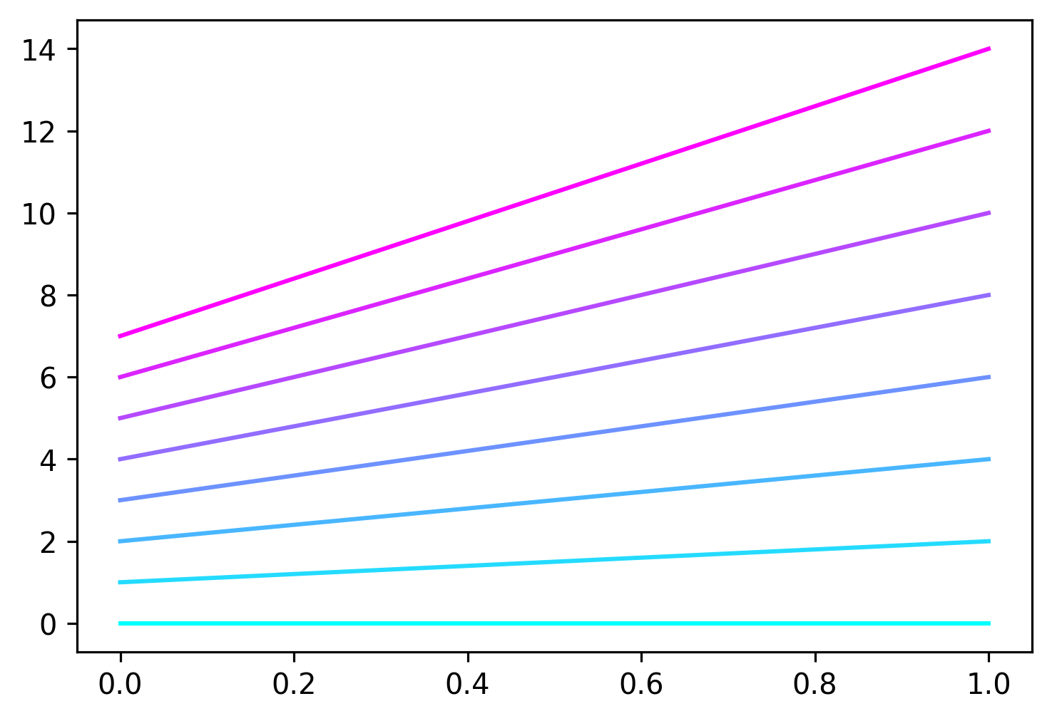
N = 8
fig, ax = plt.subplots()
set_sequential_palette(ax, 'cool', n=N)
for i in range(N):
ax.plot([0, 1], [i, 2 * i])
plt.show()
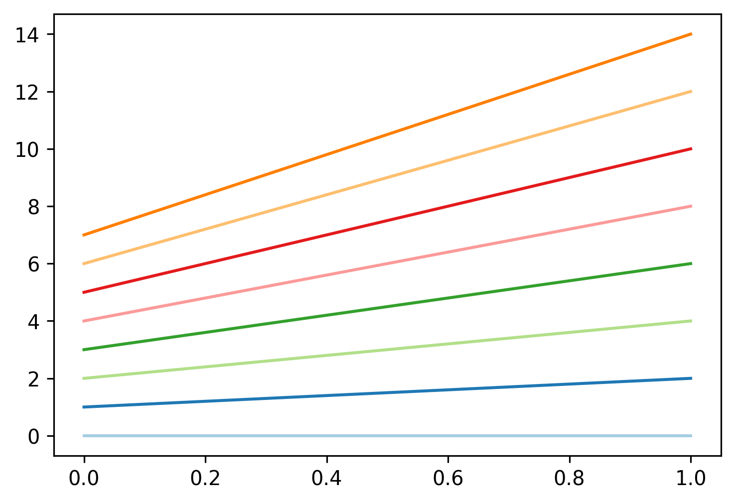
And as shown previously, for qualitative/discrete color maps, it's easier/better to just use the colors attribute and
take the first N.
N = 8
colormap = 'Paired'
fig, ax = plt.subplots()
ax.set_prop_cycle(color=mpl.colormaps[colormap].colors[:N])
for i in range(N):
    ax.plot([0,1], [i, 2*i])
plt.show()